Shooting Ball

In Houdini, there are a number of ways to fire a ball from one point, fly into the air, and have it land at a given point.

One solution would be to use a path curve, however the problem with the path follow is we cannot easily extract the point information out to get the values we want to manipulate. Path follow is usually intended to keyframe the position and that is not as procedural as one might like. To mimic realism we really are going along the distance in x in uniform steps (time), but we are traveling along the curve non-uniformly.

The second method is a simplified mathematical relationship. The arc of the ball depends on the initial velocity. This way is more mathematical (simplified of course - ignoring friction etc).

These are both available in the hip file Example shootingBall.hipnc

Method 1 — Ray SOP and User Defined Curve

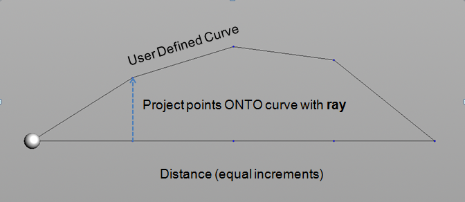
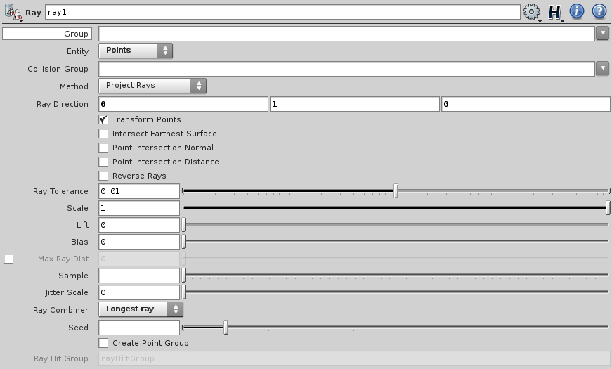
The first method is to use a ray sop and a user defined curve. The ray sop is a really quick way to get this information without doing a bunch of curve analysis. A drawn curve (just like you would use with the path follow) is used, however now you project the uniform points of units of time (ie. frames) onto the curve. This then gives you an accurate version of where the ball should be in space. You can vary the framesPerCycle (less frames, the faster it goes). This way you are guaranteed to hit the start and end and you can visually adjust the path.

The node network appears as follows:



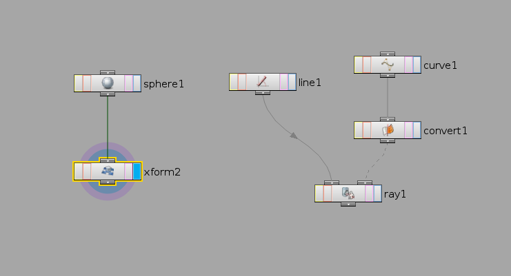
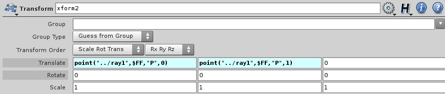
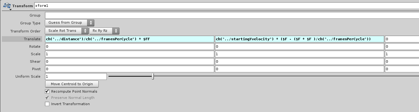
The ray sop allows you to sample the curve in a similar way to a path follow, however you are now progressing in x in equal increments (such as $FF). For example, the expressions in the transform node are:



The ray sop settings are as follows:

Method 2 — Simplified Mathematical Relationship

Math behind shooting a ball with distance, frames and vertical velocity control

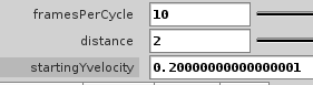
The second method is a simplified mathematical relationship. The arc of the ball depends on the initial velocity. This way is more mathematical (simplified of course — ignoring friction etc). The arc of the curve that it follows will be dependent on the startingYvelocity. This is much the way a ball would fly into the air. Using distance, starting velocity in the y direction (which at the top the change in y will be zero, and then decrease), and framesPerCycle. Again framesPerCycle will control the speed.

The second method is based on the fact that the change in x, that is to say, dx = distance / frames and we can integrate over this to find the value at a given frame.

If you take the integrals to find x and y you will get the formula for x and y at a given frame assuming it is "frames" long.
x (frame) = distance/frames * frame
y (frame) = startingYvelocity * (frame - (frame * frame)/frames)

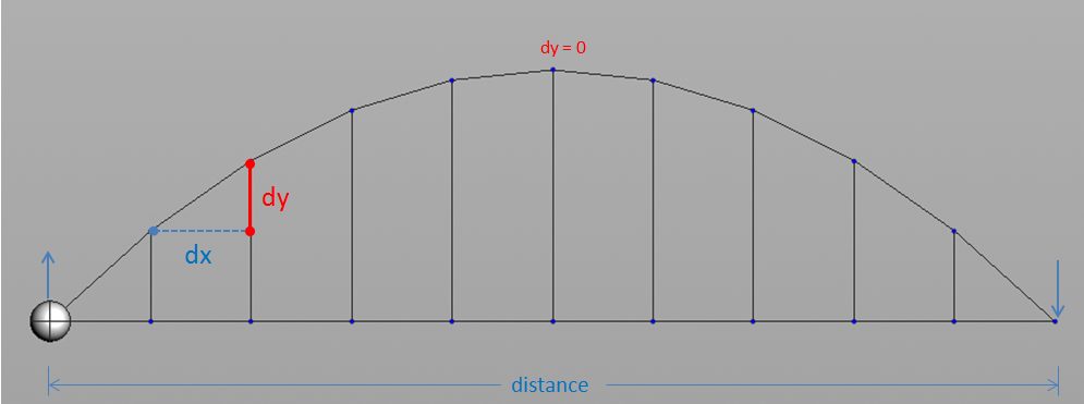
The diagram above shows equal increments in x, so if we use the frames as the total time, the change in x is:
Note that frames is the total number of frames and frame is the current frame.

dx = distance / frames

The change in y is equal to the y component of the starting velocity, call it vy, minus the current frame times (2 * vy) / frames. Written as:

dy = vy - frame * (2 * vy) / frames

This makes sense since dy(0) = vy, dy(1/2 frames) = 0 at the top of the curve, and dy(frames) = -vy.

Integrating to find x(frame):

x(frame) = ∫ distance/frames * dframe

        = distance/frames * frame

Integrating to find y(frame):

y(frame) = ∫ (vy - frame * (2 * vy) / frames) * dframe

        = vy - frame - 1/2 * frame^2 * 2 * vy / frames

        = vy - frame - frame^2 * vy/frames

        = vy (frame - frame^2/frames)

This gives us the formulas for the current frame.

The expressions in the transform node are:



Where the parameters are: